您的购物车目前是空的!
1. 神经网络概述
分类 未分类

1.背景
- 在上一章中,我们已经系统讲解了前馈神经网络训练过程的数学原理,包括网络设计、损失计算、偏导数计算及参数更新等核心机制。
-
本章将基于这些原理,采用
Python编写代码,通过逐步计算(顺序编码)的方式实现完整的训练流程,重点展示每一个数学步骤如何在代码中具体落地。 - 在下一章中,我们将进一步使用矩阵运算的方式实现同样的训练过程,以提升实现效率并更贴近现代深度学习框架的计算模式。
2.样本数据
-
总共
10个样本数据,输入数据x只有一个特征值,输出数据y也只有一个特征值。
X = [-10.0, -7.78, -5.56, -3.33, -1.11, 1.11, 3.33, 5.56, 7.78, 10.0]
Y = [0.9413, 1.1254, 1.2278, 1.1222, 1.1027, 0.4576, -0.1547, 0.4595, 0.9119, 0.9897]3.设计神经网络
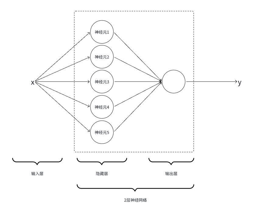
3.1.隐藏层设计
-
使用
python代码实现5个神经元,即5个【线性函数+Sigmoid激活函数】
$$\tag1 h_1 = \sigma(w_1x+b_1)$$
$$\tag2 h_2 = \sigma(w_2x+b_2)$$
$$\tag3 h_3 = \sigma(w_3x+b_3)$$
$$\tag4 h_4 = \sigma(w_4x+b_4)$$
$$\tag5 h_5 = \sigma(w_5x+b_5)$$
使用
PyTroch深度学习框架,PyTorch库提供深度学习相关的工具。
-
隐藏层实现为
HiddenLayer类:-
__init__:随机初始化\(w_i,b_i \)函数参数,使用randn获得0-1的随机数的一维张量。 -
forward:隐藏层的实际计算方法,实现5个【线性+激活】函数。
-
class HiddenLayer():
    def __init__(self):
        self.w1 = torch.randn(1, requires_grad=True)
        self.w2 = torch.randn(1, requires_grad=True)
        self.w3 = torch.randn(1, requires_grad=True)
        self.w4 = torch.randn(1, requires_grad=True)
        self.w5 = torch.randn(1, requires_grad=True)

        self.b1 = torch.randn(1, requires_grad=True)
        self.b2 = torch.randn(1, requires_grad=True)
        self.b3 = torch.randn(1, requires_grad=True)
        self.b4 = torch.randn(1, requires_grad=True)
        self.b5 = torch.randn(1, requires_grad=True)

    def forward(self, x):
        h1 = torch.sigmoid(self.w1*x + self.b1)
        h2 = torch.sigmoid(self.w2*x + self.b2)
        h3 = torch.sigmoid(self.w3*x + self.b3)
        h4 = torch.sigmoid(self.w4*x + self.b4)
        h5 = torch.sigmoid(self.w5*x + self.b5)

return h1,h2,h3,h4,h53.2.输出层设计
-
使用
python代码,实现对隐藏层输出的5个结果的权重相加。
$$\tag1 \hat{y} = a_1h_1+a_2h_2+a_3h_3+a_4h_4+a_5h_5$$
-
隐藏层实现为
OutputLayer类:-
__init__:随机初始化\(a_i \)参数 -
forward:输出层的实际计算方法,合并隐藏层的5个结果。
-
class OutputLayer():
    def __init__(self):
        self.a1 = torch.randn(1, requires_grad=True)
        self.a2 = torch.randn(1, requires_grad=True)
        self.a3 = torch.randn(1, requires_grad=True)
        self.a4 = torch.randn(1, requires_grad=True)
        self.a5 = torch.randn(1, requires_grad=True)

    def forward(self, h1, h2, h3, h4, h5):
        y_pred = self.a1*h1 + self.a2*h2 + self.a3*h3 + self.a4*h4 + self.a5*h5
return y_pred4.训练代码
- 超参数设定
# 学习率
lr = 0.01

# 训练次数
epochs = 50

# 训练批次
batch_size = 1- 设定损失函数
- 使用预测值和样本输出值的方差作为损失值,训练目的即降低方差,使其接近0。
def loss_func(y_pred, y):
return (y_pred - y).pow(2)- 初始化网络层
hidden_layer = HiddenLayer()
output_layer = OutputLayer()- 循环迭代
-
样本输入数据
x先经过hidden_layer处理,之后在output_layer进行权重合并。 -
将预测结果
y_pred和样本y使用loss_func函数计算差值。 -
对
loss进行backward反向传播,即可自动计算参数\(a_i,w_i,b_i\)的偏导数。
backward()是由PyTorch提供的快速计算偏导数的方法。对loss进行backward()后所有参与计算loss值的变量(\(a_i,w_i,b_i\))会自动计算各自对loss的偏导数,并将计算偏导数结果保存到各自的.gard变量中。
# 训练
for epoch in range(epochs):
    total_loss = 0

    for x, y in zip(X, Y):
        # 前向传播
        h1, h2, h3, h4, h5 = hidden_layer.forward(x)
        y_pred = output_layer.forward(h1, h2, h3, h4, h5)

        # 计算损失
        loss = loss_func(y_pred, y)

        total_loss += loss.item()

        # 反向传播
        loss .backward()

        # 更新参数
        with torch.no_grad():
            hidden_layer.w1 -= lr * hidden_layer.w1.grad
            hidden_layer.w2 -= lr * hidden_layer.w2.grad
            hidden_layer.w3 -= lr * hidden_layer.w3.grad
            hidden_layer.w4 -= lr * hidden_layer.w4.grad
            hidden_layer.w5 -= lr * hidden_layer.w5.grad

            hidden_layer.b1 -= lr * hidden_layer.b1.grad
            hidden_layer.b2 -= lr * hidden_layer.b2.grad
            hidden_layer.b3 -= lr * hidden_layer.b3.grad
            hidden_layer.b4 -= lr * hidden_layer.b4.grad
            hidden_layer.b5 -= lr * hidden_layer.b5.grad

            output_layer.a1 -= lr * output_layer.a1.grad
            output_layer.a2 -= lr * output_layer.a2.grad
            output_layer.a3 -= lr * output_layer.a3.grad
            output_layer.a4 -= lr * output_layer.a4.grad
output_layer.a5 -= lr * output_layer.a5.grad- 循环结束后将最终的\(a_i,w_i,b_i\)参数值进行保存,至此完成整个训练过程。
5.推理代码
-
使用训练好的参数对实际问题进行预测,这里直接画出
x在[-10,10]的1000点上的计算值。
# 绘制预测结果
plt.figure(figsize=(10, 6))

# 生成更密集的点来绘制平滑的预测曲线
x_dense = np.linspace(min(X), max(X), 1000)
y_pred_dense = []

# 计算预测值
for x in x_dense:
    with torch.no_grad():
        h1, h2, h3, h4, h5 = hidden_layer.forward(torch.tensor(x, dtype=torch.float32))
        y_pred = output_layer.forward(h1, h2, h3, h4, h5)
        y_pred_dense.append(y_pred.item())

# 绘制实际数据点
plt.scatter(X, Y, color='red', label='实际数据点', zorder=5)

# 绘制预测曲线
plt.plot(x_dense, y_pred_dense, color='blue', label='模型预测', linewidth=2)

# 设置图表属性
plt.title('神经网络拟合结果', fontsize=14)
plt.xlabel('输入 x', fontsize=12)
plt.ylabel('输出 y', fontsize=12)
plt.grid(True, linestyle='--', alpha=0.7)
plt.legend(fontsize=10)

# 显示图表
plt.show()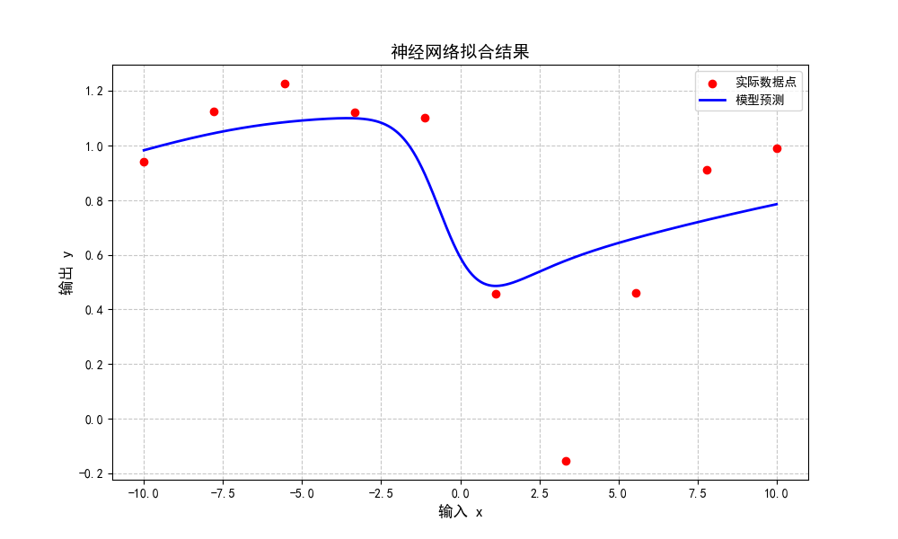
6.附件:完整代码
import torch
import numpy as np
import matplotlib.pyplot as plt

# 设置matplotlib中文字体
plt.rcParams['font.sans-serif'] = ['SimHei']  # 用来正常显示中文标签
plt.rcParams['axes.unicode_minus'] = False  # 用来正常显示负号

# 输入数据
X = [-10.0, -7.78, -5.56, -3.33, -1.11, 1.11, 3.33, 5.56, 7.78, 10.0]

# 输出数据
Y = [0.9413, 1.1254, 1.2278, 1.1222, 1.1027, 0.4576, -0.1547, 0.4595, 0.9119, 0.9897]

# 随机初始化参数

class HiddenLayer():
    def __init__(self):
        self.w1 = torch.randn(1, requires_grad=True)
        self.w2 = torch.randn(1, requires_grad=True)
        self.w3 = torch.randn(1, requires_grad=True)
        self.w4 = torch.randn(1, requires_grad=True)
        self.w5 = torch.randn(1, requires_grad=True)

        self.b1 = torch.randn(1, requires_grad=True)
        self.b2 = torch.randn(1, requires_grad=True)
        self.b3 = torch.randn(1, requires_grad=True)
        self.b4 = torch.randn(1, requires_grad=True)
        self.b5 = torch.randn(1, requires_grad=True)

    def forward(self, x):
        h1 = torch.sigmoid(self.w1*x + self.b1)
        h2 = torch.sigmoid(self.w2*x + self.b2)
        h3 = torch.sigmoid(self.w3*x + self.b3)
        h4 = torch.sigmoid(self.w4*x + self.b4)
        h5 = torch.sigmoid(self.w5*x + self.b5)

        return h1,h2,h3,h4,h5

class OutputLayer():
    def __init__(self):
        self.a1 = torch.randn(1, requires_grad=True)
        self.a2 = torch.randn(1, requires_grad=True)
        self.a3 = torch.randn(1, requires_grad=True)
        self.a4 = torch.randn(1, requires_grad=True)
        self.a5 = torch.randn(1, requires_grad=True)

    def forward(self, h1, h2, h3, h4, h5):
        y_pred = self.a1*h1 + self.a2*h2 + self.a3*h3 + self.a4*h4 + self.a5*h5
        return y_pred

# 损失函数
def loss_func(y_pred, y):
    return (y_pred - y).pow(2)

def main():
    # 学习率
    lr = 0.01
    # 训练次数
    epochs = 50
    # 训练批次
    batch_size = 1

    # 初始化网络
    hidden_layer = HiddenLayer()
    output_layer = OutputLayer()

    # 训练
    for epoch in range(epochs):
        total_loss = 0

        for x, y in zip(X, Y):
            # 前向传播
            h1, h2, h3, h4, h5 = hidden_layer.forward(x)
            y_pred = output_layer.forward(h1, h2, h3, h4, h5)

            # 计算损失
            loss = loss_func(y_pred, y)

            total_loss += loss.item()

            # 反向传播
            loss.backward()

            # 更新参数
            with torch.no_grad():
                hidden_layer.w1 -= lr * hidden_layer.w1.grad
                hidden_layer.w2 -= lr * hidden_layer.w2.grad
                hidden_layer.w3 -= lr * hidden_layer.w3.grad
                hidden_layer.w4 -= lr * hidden_layer.w4.grad
                hidden_layer.w5 -= lr * hidden_layer.w5.grad

                hidden_layer.b1 -= lr * hidden_layer.b1.grad
                hidden_layer.b2 -= lr * hidden_layer.b2.grad
                hidden_layer.b3 -= lr * hidden_layer.b3.grad
                hidden_layer.b4 -= lr * hidden_layer.b4.grad
                hidden_layer.b5 -= lr * hidden_layer.b5.grad

                output_layer.a1 -= lr * output_layer.a1.grad
                output_layer.a2 -= lr * output_layer.a2.grad
                output_layer.a3 -= lr * output_layer.a3.grad
                output_layer.a4 -= lr * output_layer.a4.grad
                output_layer.a5 -= lr * output_layer.a5.grad

                # 清零梯度,否则每次loss.backward()会累计偏导数计算结果
                hidden_layer.w1.grad.zero_()
                hidden_layer.w2.grad.zero_()
                hidden_layer.w3.grad.zero_()
                hidden_layer.w4.grad.zero_()
                hidden_layer.w5.grad.zero_()

                hidden_layer.b1.grad.zero_()
                hidden_layer.b2.grad.zero_()
                hidden_layer.b3.grad.zero_()
                hidden_layer.b4.grad.zero_()
                hidden_layer.b5.grad.zero_()

                output_layer.a1.grad.zero_()
                output_layer.a2.grad.zero_()
                output_layer.a3.grad.zero_()
                output_layer.a4.grad.zero_()
                output_layer.a5.grad.zero_()

        print(f"Epoch {epoch+1}, Average Loss: {total_loss/len(X):.6f}")

    plot_result(hidden_layer, output_layer)

def plot_result(hidden_layer, output_layer):
    # 绘制预测结果
    plt.figure(figsize=(10, 6))

    # 生成更密集的点来绘制平滑的预测曲线
    x_dense = np.linspace(min(X), max(X), 1000)
    y_pred_dense = []

    # 计算预测值
    for x in x_dense:
        with torch.no_grad():
            h1, h2, h3, h4, h5 = hidden_layer.forward(torch.tensor(x, dtype=torch.float32))
            y_pred = output_layer.forward(h1, h2, h3, h4, h5)
            y_pred_dense.append(y_pred.item())

    # 绘制实际数据点
    plt.scatter(X, Y, color='red', label='实际数据点', zorder=5)

    # 绘制预测曲线
    plt.plot(x_dense, y_pred_dense, color='blue', label='模型预测', linewidth=2)

    # 设置图表属性
    plt.title('神经网络拟合结果', fontsize=14)
    plt.xlabel('输入 x', fontsize=12)
    plt.ylabel('输出 y', fontsize=12)
    plt.grid(True, linestyle='--', alpha=0.7)
    plt.legend(fontsize=10)

    # 显示图表
    plt.show()

if __name__ == "__main__":
    main()
发表回复